Basic Excel Pivot Table

To better understand the concept of pivot tables and their role in reporting and data analysis, I did some online research before attending the lecture on Pivot Tables. This is what I found:

What is a Pivot Table in Excel?

A Pivot Table gathers all the data in an Excel spreadsheet (or range of a spreadsheet) and presents a summary of this data in a table. This table allows you to see, at a glance, information such as:

• The number of items of each type;
• The sum of a data column, broken down into data types;
• The average of a data column, broken down into data types.

A step-by-step guide of how to create a basic Excel Pivot Table:

A step-by-step guide is helpful in creating a pivot table for someone new to this concept. When I listened the lecture, I was not able to reproduce it as I did not have any prior knowledge of pivot tables. I had to research further to understand the basics of pivot table. In the following example of creating a basic pivot table, I am going to reference to the excel file which was provided with the lecture.

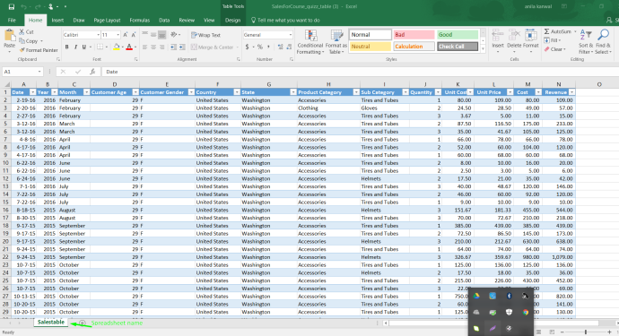
Following is a screen shot of the data set provided in the excel file.

This example will show a pivot with “Country “as rows, “Month” as columns, and “Revenue” as values, and it is filtered by “Years”.

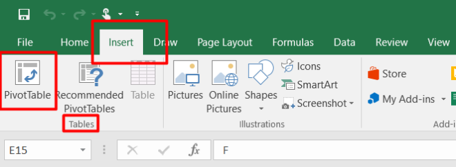
Select a cell or click anywhere in the data range to be used for pivot table, excel will automatically identify, and select the whole data range for the Pivot Table. On ribbon, click -> “Insert” -> “Pivot Table” (which is a part of “Table” grouping).

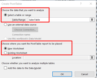
Create PivotTable dialogue box will be opened. There are two major portions of this dialogue box.

1. Name of the table which is SalesTable in this example (or a data range if table is not given a name).
2. Place where we want pivot table to be placed.

(Note: Selected options are default, we can change them as/if needed)

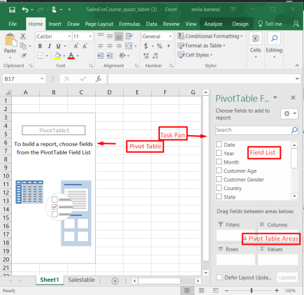
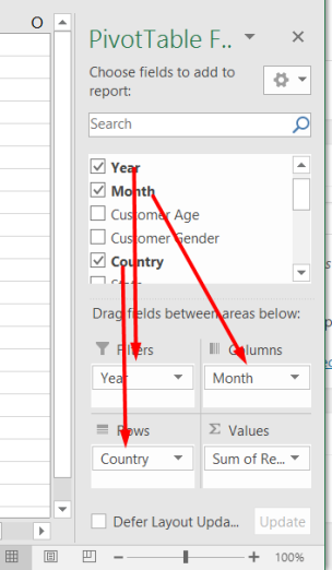
 Now, there will be an empty Pivot Table on the new sheet with the ‘Pivot Table Field List’ task pane, which contains several data fields (columns of original data table).

Within the pivot table field list:

• Drag “Country” into the “Rows” area
• Drag “Month” into the “Column” area
• Drag “Revenue” into the “Values” area
• Drag “Years” into the “Filter” area

 

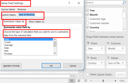
 Note: Make sure that the value in the ‘Σ Values’ section reads “Sum of Revenue” and not “Count of Revenue”. By default, “Values” area shows “Sum” if the the inserted filed/column has numeric values. Otherwise, it will default to “Count of Revenue” if the inserted filed/column has non-numeric or blanks values.

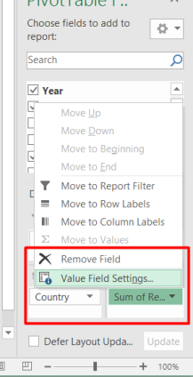
∑ Values settings can be changed according to the need by left clicking and selecting ‘value field setting’.

 

The Pivot table will be populated with the values as following:

Take care out there, see you soon with some more information on Pivot Tables.